| Ralph Vince* |
| Corresponding Author: 405 Lexington Ave - The Chrysler Building, 26th Floor, New York NY 10174, USA. |
| Received: 22 May 2020; Revised: June 28, 2020; Accepted: 25 May 2020 |
| Share : |
2749
Views & Citations1749
Likes & Shares
Often,
geometric growth maximization techniques as presented by (Kelly, 1956; Thorp,
1962; Vince et. al., 2019 & Vince, 1990) have looked only at such ambits
where the implementor was concerned with maximizing growth, or more generally,
situations where growth was beneficial to the implementor (Vince, 2013; Vince,
2015).
In
this paper we examine using these techniques on geometric growth functions
where the implementor benefits from diminished growth. Certain geometric growth
functions accruing against the public, often characterized as “growing out of
control,” typically meet this criterion. These often include medical costs, the
growth of populations (e.g., bacteria) or pathogenic infections in a
population, infected cells in an organism, or even the growth of cumulative
national debt.
Finally,
we demonstrate the technique upon this notion of the growth rate of a nation’s
cumulative debt. Heretofore, debt reduction has been considered along the
one-dimensional tug-of-war between reducing government services or increasing
taxes. The technique presented, albeit very simple, provides a
politically-agnostic means of debt-reduction. We provide further examples of
potential applications in terms of mitigating malevolent cellular growth and
concerns for applying the material in the spread of pathogenic outbreaks.
Interaction
with stochastic, time-series data is implicitly an exercise in geometric growth
maximization. If we consider a random stream of outcomes over time, in almost
every case, resources available to allocate to the immediate outcome is an
unavoidable result of the cumulative trail of outcomes to that point in time.
The results compound. There exists not-so-common exceptions to this compounding
effect (consider a retiree who receives a pension he does not need in order to
meet his expenses, which he chooses to wager on a particular gamble with each pension
distribution), but in most cases compounding is implicit, and we restrict our
discussion to such ever-prevalent cases.
Maximization of results from stochastic, time-series data has a long history, beginning with (Bernoulli, 1738) who, in 1738, provides the first known reference to “geometric mean maximization”.
This
1738 paper, written in Latin containing the first known reference to geometric
mean maximization, is translated into English in 1954 (Bernoulli, 1738).
In
his 1956 paper, (Kelly, 1956) showed how Shannon's “Information Theory”
(Shannon, 1948) could be applied to the problem of a gambler who has inside
information in determining his growth-optimal bet size.
Six
years later, (Thorp, 1962) applies the concept to the actual gambling situation
presented in the game of Blackjack. Thorp would later provide closed-form
solutions.
In
1990, (Vince, 1990) provides a solution for capital market applications, and by
2019 in (Vince & Optimal, 2019) provides the full (non-asymptotic,
non-instantaneous) solution for geometric mean maximization for all conditions.
Other
avenues where other variants of geometric growth amplification are shown to be
“optimal”, for criteria other than outright maximization appear in (Lopez,
Vince & Zhu, 2019; Vince & Zhu, 2013; Vince & Zhu, 2015).
Yet everything up to such a point refers to geometric growth as something that is desired, beneficial, and seeks ways to maximize the benefit derived from such streams of stochastically-generated outcomes.From (Vince & Optimal, 2019) we find, in simplest form, geometric growth is maximized for a single stream (as opposed to multiple, simultaneous streams) of Q stochastic outcomes[1], x, asymptotically (i.e., as the number of trials approach infinity), by that fraction of the total cumulative pool at any i, by that value for f (0…1) which maximizes the geometric mean outcome, G:
G
(f) = Q √( ∏i=1Q1 + f (-xi
⁄ min (x1…xQ
))) (1)
As mentioned, the value for f which maximizes G(f) in (1) is asymptotic with respect to ever-greater Q. When Q=1, if the probability weighted mean value for x is positive, then G will be maximized at a value of 1, and this will approach the value given in (1) asymptotically with ever-higher Q. If the probability-weighted mean value for x is zero or less, then the function for G is maximized at f=0, and remains for all possible values of Q.
Where:
G =the
probability-weighted geometric mean outcome of the stream of outcomes.
Q = the number of
outcome events in the stream of outcomes.
f =the constant
fraction of the total pool of resources allocated on each outcome in the
stream.
xi =an
individual result of the i’th
outcome event.
n.b. min (x1…xQ) must be a
negative number, otherwise the value for f
which maximizes G(f)is 1
for all possible values of Q.
Let us examine a simple stream of outcomes which are binomially-distributed, such as the results of a coin toss. We will assign a value of 2 if the coin lands favorably to us, and a value of -1 if it lands the opposite way, unfavorable to us.
Thus,
if one seeks to find that value for f which maximizes G(f),
equation (1) is properly expressed as:
limQ→∞ G (f) = Q √ (∏i=1Q 1+ f (-xi ⁄ min x1…xQ )) (1)
The non-asymptotic
formulation, that is, the determination of the growth-optimal value for f
for a finite-length stream of stochastic outcomes (Q <∞) is given in
(Vince, 1995).
It
is important to note that growth gets ever greater as f increases from 0
to its asymptotically growth-optimal value between 0 and 1, as given in
equation (1) and then decreases. That is, asymptotically, as Q gets
ever-greater, growth is reduced with ever-greater values for f beyond
that given in equation (1).
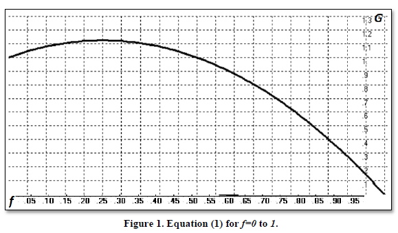
Thus,
we find for our 2: -1-coin toss, by Equation (1), we see that geometric growth
of our pool is achieved as Q, the number of trials, gets ever-greater,
at f=.25 as we see in Figure 1.
If
we took this stream of outcomes, 2, -1, where Q=2, and applied
the values to (1), we would find that G(f) is maximized at f=.25
where G (.25) =1.06066. Thus, if
we were to wager .25 of our entire pool on each coin toss in sequence,
regardless of sequence, we would maximize our gains as Q got ever
greater.
G (.25) = Q √ (1+.25(-2 ⁄ -1) x (1+.25 (- -1 ⁄ -1)
G (.25) = Q√ (1.5 x .75)
G (.25) = 1.06066
This value, 1.06066, the geometric mean return outcome, represents the multiple we would make on our pool, on average, with each coin toss, with each event, since we are “reinvesting” after each toss (i.e., our pool, from which we take a fraction, f, of to wager on the next toss, is the cumulative result of the outcomes of all subsequent tosses). This number is necessarily less than the “average” (the arithmetic mean return per event): A(f) = ∑i=1Q1 + f (-xi ⁄ min (x1…xQ)) / Q (2)
Just
as there is a geometric mean outcome, G, for any value for f, so
too is there an arithmetic mean outcome, we shall designate as A, and
for our 2:-1 coin toss, where f=.25, we find G=1.06066 and, from
(2), A = 1.125.
SEEKING GEOMETRIC GROWTH ATTENUATION OR
DIMINISHMENT
We
shall now play devil’s advocate, where our goal, when faced with the growth of
such streams which appear with a geometric growth amplifier innate to them, is
to attenuate rather than amplify such growth rates. Typically, the literature
on the matter has previously been focused on maximizing growth in a stream of
stochastic outcomes. Now, we shall examine ways, first introduced in (Vince,
1995), to use the ideas to reduce geometric growth in stochastic outcomes. The
real-world is rife in systems where we would desire this. Among these types of phenomena are things
like the growth of bacteria in a petri dish, the spread of infectious disease
in a population of organisms, the spread of pathogenic cells within an
individual organism, or even, say, the growth rate of a nation’s cumulative
debt. The same mathematical formulations are at work as when we desire growth.
The
problem is, in looking for diminishment in these aforementioned types of
geometric growth situations where we seek diminishment, what is the f
value? Clearly, there is no such governing value of the growth rate of a
nation’s aggregate debt’s rate of growth or in other situations where we desire
geometric growth attenuation or diminishment. Where do we obtain an available
parameter to affect the formulation which belies the geometric growth function
here?
Just
as there is a geometric mean outcome, G, for any value for f, so
too is there an arithmetic mean outcome, we shall designate as A, and a
variance, we shall designate as V, to the stochastic stream of outcomes.
For our 2: -1-coin toss, we thus
have corresponding values of 1.06066 for G, 1.125 for A, and
.140625 for V, the population variance. Since standard deviation,
SD, is simply the square root of variance, we can express this SD = 0.375.
We can thus summarize as
follows for this simple, binomial case:
f
= 0.25
G
= 1.06066
A
= 1.125
SD = 0.375
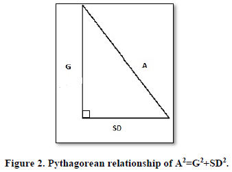
Serendipitously, as demonstrated in (Henry, 1959), these values comport perfectly to the Theorem of Pythagoras as:
A2 = G2 + SD2 (3)
Our
goal here, as the advocate of the devil, is to seek geometric growth
diminishment. Thus, we seek to make the value for G be as small as possible, as
it can be said that the growth of the pool after Qevents is GQ.
With Q as a given, any reduction in
SD that can exceed an offsetting increase in A will reduce G,
and, geometrically, the size of the pool after Q events, GQ.
From
this, we can state the following:
With respect to
growth multiples, any increase in their variance, V, affects the geometric growth
rate, G, by an amount equal to an equivalent decrease in the arithmetic average
- squared!
In
most human endeavors, when confronted with a malevolent geometric growth
function, man’s first reaction is to seek to minimize the (arithmetic) average
growth rate, A, when equally as much beneficial fruit can be derived
merely by increasing the period-on-period variance, V.
Variance,
V, or it’s square root standard deviation, SD, depending on the
function, often tend to move with respect to A in a non-linear manner; i.e.,
often, as A increases, so too does SD, with the latter increasing
at a faster rate. This leads to the familiar peak in G (0...1) such as
we see in Figure 1.
However,
in many malevolent, naturally occurring growth functions, we are able to effect
SD, to increase SD, without a corresponding increase in A.
If, in Figure 2, one increases SD without a corresponding
increase in A of the same increase as being applied to SD, then G
is necessarily smaller.
Any increase in the base of a right-angled triangle without any
equivalent or greater increase in the hypotenuse will reduce the vertical leg,
will achieve our goal, will diminish growth.
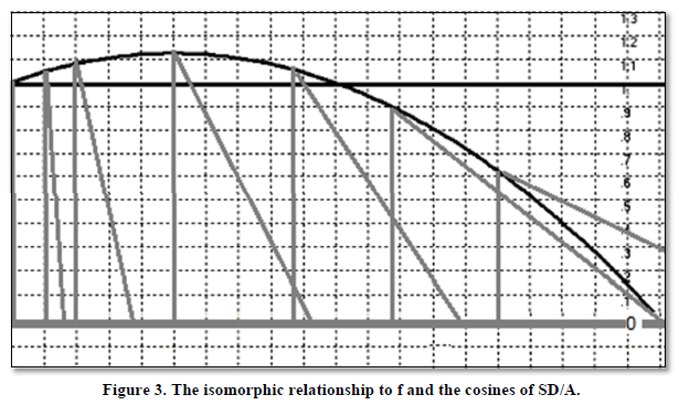
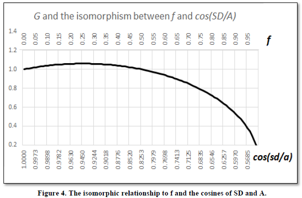
We thus find there exists an isomorphism
between the f value illuminated in Section 1 and the cosine of the standard
deviation and mean of the period-on-period growth in a stream of malevolent
stochastic events. Graphically, this is depicted in Figure 3.
In
the simplest case, if we disregard A varying with respect to V,
we can unequivocally then state that for constant A, that is if we can
hold A constant, any increase in V reduces G. If A
increases with respect to V, we witness a curve with a peak in the
horizontal range of values beyond which geometric growth begins to diminish.
Figures
1, 3, and 4
show where A varies with changing V. This is not necessarily the
case however, as often variance can be increased without increasing the
arithmetic average in a sequence, particularly those of “malevolent” character
where our directed efforts can be used to increase variance. When A does
not increase with increasing V, the peak of the curve is at its
left-most point, that point where f=0 and cos(SD/A) = 1 (i.e.,
the “base” of the triangle is zero-- is it no longer a triangle at this point
but merely a vertical line).
Thus,
there exists two important points in the range of values of “directed effort,”
either with respect to percentage of a resource we allocate to the multiples of
a stream of stochastic outcomes or the cosines of the standard deviation to
means of these outcomes.
The
two points are portrayed in Figure 5. Working from the left, the first
of these points is that point where the curve begins descending, where the
slope of the first derivative turns negative. This represents that point where
as f (the “fraction allocated”) increases further, or the size of
the base (V) relative to the hypotenuse (A) increases further, geometric
growth becomes less.
Of note, if A does not increase
with increasing V, the peak of the curve is at the leftmost bound, and
hence this first geometrically significant point is immediately to the right of
the leftmost bound by an infinitesimally small amount; i.e., as soon as f
or V increases, G decreases.
The
second important point is that point where the value for G crosses 1 to the downside, and we
refer to this point as ψ. Any
given number multiplied by a number less than 1 will have a lower product than
the given number. Repeatedly multiplying the resultant product by a number less
than 1 will cause the resultant products to get ever-closer to zero. A value
for G
less than unity will cannibalize itself as more periods accrue.
From this, we can see that Sir Ronald Fisher’s
fundamental theorem of natural selection (Ronald, 1930), which states:
“The rate of increase in fitness of any organism at
any time is equal to its genetic variance in fitness at that time.”
Provides
only a partial explanation; it consists of looking at the natural world as it
exists in nature, to the “left” of the peak where A increases with
increasing V. However, by increasing this variance beyond the peak, we
can see that such fitness diminishes with further increases in variance, and at
the point ψ extinction is ultimately assured.
In
the natural world, the point to the right of the peak is obscured; too much
variance in fitness, and the organism no longer exists.
The
Pythagorean relationship in (3), expressed between the arithmetic mean of
growth multiples and the geometric mean and standard deviation of these
multiples, is exact if the stream of multiples is binomially distributed.
Other
measures for estimating geometric growth have been proposed and can sometimes
be more accurate and deserve discussion.
In (de La Grandville, 1989) speaks of misconceptions in estimating long-term returns and refers to the popularity of one widely held formula for estimating geometric returns as being “approximately equal to the arithmetic average minus half of the variance,” or:
G = A – V / 2 (4)
Another formula, common in quantitative finance for estimating the geometric mean return which provides an exact estimate when the returns are lognormally-distributed is:
G = A ⁄ √1+V x A-2 (5)
Generally
(3) will be less than (5). Typically, (3) is not greater than the actual G for
most real-world, non-binomially-distributed data sets.
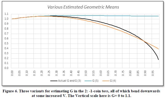
All
examples for estimating the geometric return, Equations (3), (4), and (5),
generally work for any return sample, and establish approximate relationships
between the geometric and arithmetic averages and the variance. These formulas
are all based on Taylor series expansions up to the second degree.
The
question as to “Which is best?” is a debate for another paper as all three of
these approximations provide values for G which begin decreasing at some
level of V in the domain of values for V. All three
approximations see the curve for G bend downwards at some point as V
increases.
For
various, real-world data sets of various distributions, we find that the value
for Equation (3), though for some data sets not the best estimation for G
of the three, is never the worst estimation for G of the three
equations. For this reason alone, in the real-world where often, the
distribution of a priori data is unknown, Equation (3) is in fact, the
best estimator for G.
Finally, when we get into the
lower values for the cosine of SD over A, that is, when V
begins to get larger with respect to A, when the points of geometrical
significance are encountered, particularly by the time V is at a
critical enough value to encounter the point ψ, Equations (4) and (5)
are unable to keep pace. For the 2: -1-coin toss, this becomes evident in Figure
6 and 7.
This is central
to our argument, that at some point of higher V, G is decreased. All three values
for estimating G support this contention. However, we find that using the
Pythagorean estimate of Equation (3) to be the best fit for our purposes and
can be certain, regardless of the distribution of outcomes we will be applying
it to, it will never be the worst estimate, and most importantly, that by
increasing variance, at some increased value (perhaps immediately) we will
begin to see reductions in G.
Examples
Example
1 – A politically agnostic means of deficit reduction
For the sake of illustration, we
demonstrate the method in a simplified example using a binary stream of
stochastic outcomes. As pointed out, this stream need not necessarily be binary-distributed,
we merely use it for simplicity’s sake to illustrate the method.
We
examine the period-on-period percentage changes in growth and re-express these
as a Multiple on the aggregate of the prior period as 1 plus the
period’s percentage growth.
We
further introduce in this example the notion of Constant
Dollars Forward, which represents the
amount of cumulative debt (it's initial principal plus its service) represented
by an individual silo of one million going forward, as of a given start
date. Thus, each period forward will see new, non-debt-service borrowing that
is not addressed here. Rather, this addresses the debt-service cost of one million
in debt into the future.
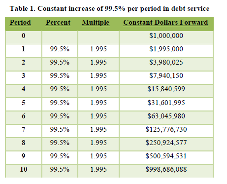
Our first example sequence shows a constant increase of 99.5% per
period in debt service, which appears as follows for ten periods (Table 1).
Since the stream is the same 99.5% from one period to the next,
the arithmetic average, A, and the geometric average, G, of the
period-on period multiples is identical at 1.995. Thus, for this constant
growth sequence, we have:
A=1.995;
V=0
SD=0
G=1.995
There is no variance in this first sequence. In this example, we
are able to keep A constant while increasing variance, V, and so
the introduction of any variance – that is, increasing the base of a
right-angled triangle while holding the length of the hypotenuse constant, must
result in a shorter vertical leg, G.
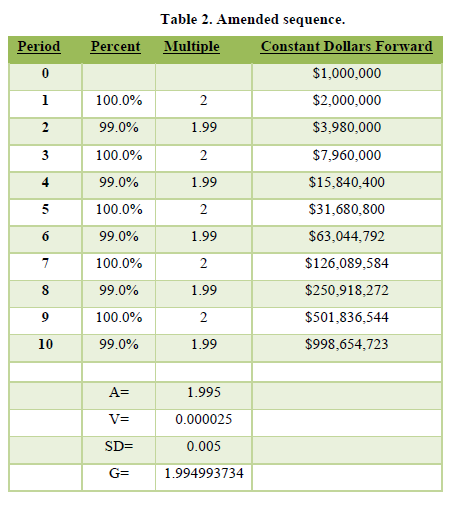
We see this when we amend the sequence to be simply the
alternating binary distribution of 100% and 99% increases (Table 2).
The introduction of variance,
even as small as .000025 in the period-on-period growth multiples, shows a
growth rate diminished from 1.995 when variance, V, was 0 to 1.994993734
even though the (arithmetic) average period-on-period growth multiple remains
at 1.995, or an average gain of 99.5% per period. The cumulative growth at the
end of the period is reduced simply by the introduction of variance.
Unlike Figures 1, 3, and 4, where the arithmetic average
growth rate, A, increased with respect to variance, V, and hence
the geometric average growth rate, G, had a peak farther down range than
the leftmost values on the horizontal axis of f=0 or cos(SD/A)=1,
when A does not increase with increased V (as may be the case in
real-world applications of directed efforts to increase period-on-period
variance) we find G achieves its peak at the leftmost values and
decreases from there with increased directed effort.
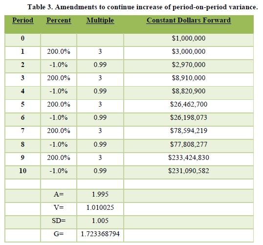
To continue to increase this period-on-period variance we find,
still holding the (arithmetic) average growth per period at 99.5%, represented
as the binary sequence 200, -1 (Table 3).
The period-on-period growth rate, G, is further reduced to
1.723368794, and the total growth of the starting amount of $1,000,000 is now
cut to less than 1/4th over ten periods of what it was at no
period-on-period variance.
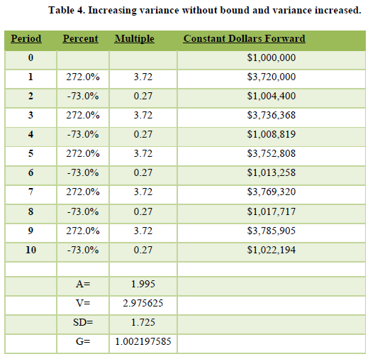
Assuming we can increase variance without bound, we examine the
sequence 272, -73, which shows a period-on-period average growth rate, A, of
1.995 and variance, V, increased to 2.975625 (Table 4).
Notice the Constant Dollars
Forward has barely increased over this sequence of 10 periods. We increase the
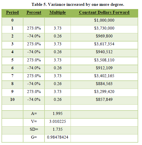
variance by one more degree at the sequence 273, -74, which still has an
arithmetic average growth rate, A, of 1.995 (Table 5).
We now see our geometric average growth rate, G, to be less than 1
at 0.98478424 for this sequence. We are now past the point ψ in terms of the
size of the base, SD, with respect to the hypotenuse, A, and the sequence has
now thus become terminal. This is so even though this sequence with an A of
1.995 thus grows at an (arithmetic) average growth of 99.5% per period. It is
still, by virtue of increased variance, terminal.
Thus, an initial silo of the growth of $1,000,000 in debt service
has been broken, and at the current average growth rate and variance will
diminish to nothing in time. Even if the average growth rate, A,
increased with respect to time, there still exists a value for V which
will cause the process to self-cannibalize.
Variance in a
nation’s cumulative debt is affected by tax policy, sporadic principal
paydowns, and rates of borrowing which are, at the shorter maturities at least,
influenced by the policies of central banks.
The
technique is politically agnostic, and there is no reason why the
period-on-period variance should not be among the primary considerations of
policymakers in such matters. These are economic gains to the population at
large that are heretofore being foregone, and would be acceptable to all
regardless of politics. Further, the matter is rife in potential fruit for
medical and pharmacological researchers.
However,
lawmakers and central bank policy makers - practitioners working to diminish a
nation’s cumulative debt, may rightfully object that such an example disregards
a plethora of real-world constraints they are up against. Similarly,
applications in the biological sciences – epidemiology, pharmacological dosing,
etc., may make similar
arguments against the technique (e.g.,
the human body could not survive the higher doses of a drug necessary in
certain periods required to increase period-on-period variance).
These are all
valid arguments. The purpose of this paper is to introduce the technique in
pure, theoretical form, that actual application left to the practitioners where
the technique might be applied. Nevertheless, with these caveats in mind
we examine a naïve, hypothetical epidemiological example of how this principle
can be useful.
Example
2 – Applications involving malevolent cellular growth
In the following example, we consider a bacterial culture in a
petri dish which we wish to diminish via an antibiotic. Let us assume the
growth rate of this culture is 1.08 per unit time. That is, it is increasing in
size by a multiple of 1.08 as each unit of time transpires. In other words, it
grows 9% in size for every unit of time.
If left untreated after ten units time, we find it has therefore
grown to:
G = 1.0810=2.158925 times its original size
Further, since it is left untreated, we determine its variance, V,
in period-on-period growth to be 0, hence, the arithmetic average growth
rate, A, is equal to 1.08 and the geometric average growth rate, G,
is per Equation (3).
Generally, antibiotics are prescribed in a manner so as to induce
a constant blood level of the antibiotic. The effect, in terms of this perspective
is that we have reduced G while leaving V still 0, and hence have obtained this
resultant lower geometric average growth rate (the only factor in this
perspective we observe directly in this example), G, solely by reducing A,
the arithmetic average growth rate.
Mathematically, we know two things:
1.
Any increase in standard deviation, SD, in period-on-period
growth (which is the square root of V) is akin to a decrease in A,
the arithmetic average period-on-period growth rate. Thus, if we can increase V
at a faster rate than A increases, we gain by this action in terms of
diminishing the average growth rate per period, G.
However, since usually
in increasing variance, the average arithmetic growth rate, A, also increases
2.
At that point where A2 – V<
1, we have reached point ψ where growth diminishment is assured by virtue of
this increase variance as shown in Figure 8.
To invoke variance, we must now administer the antibiotic in a
manner which is counter-intuitive and administer it in a manner where we do not
induce a constant blood level.
We shall assume in this hypothetical example that the prescribed
dosage for this type of bacterial culture at this level would be to apply 100
mcg of the particular antibiotic per unit time.
In maintaining a “constant blood-level” of antibiotic, by applying
the prescribed amount per unit time consistently, we have minimized
variance. This is the common manner in
which antibiotics are used.
As time elapses, we can measure the amount of culture in the petri
dish to determine the growth rate per unit time. Let us suppose we find that
after 10 units of time, our culture has shrunk to 60% of its original size from
when we began applying 100 mcg of antibiotic per unit time.
Thus, the growth rate, G, can be determined to be:
G = 0.6(1/10) = 0.6.1=.9502
Thus, applying 100 mcg per unit time sees the culture grow as the
size of the culture for the previous time unit times 0.9502.
Looking at this then, since our Variance, V, is 0, then our
arithmetic growth rate per unit time, determined from Equation (3) is:
A2 = G2 + SD2 = G2
+ V
Since
V=0, then A=G in this case, and thus A=.9502 also.
We see then that without 100mcg per unit time applied to the
culture, the culture will grow at a rate of 1.08 per unit time, and with the
100mcg constant-level antibiotic treatment, it will grow at a rate of .9502 per
unit of time (i.e., since it grows by its multiple per unit time, it
“shrinks” per unit time when the multiple is less than 1).
Given the nature of this example, we do not see the arithmetic
average growth rate directly but rather the geometric average growth rate.
Hence, we must calculate the arithmetic average growth rate from the geometric
average and the variance in period-on-period growth.
Furthermore, since we also cannot examine the variance directly
either (because the variance we witness is in period-on-period geometric
growth, not the arithmetic data underlying it from which the variance must be
determined) we are, in effect, blind to the inputs of A and V (or SD) in the
critical Equation 3 from which we determine that A2-V will give us
that growth-diminishment critical point of ψ where growth-diminishment is
mathematically assured.
Nevertheless,
we can extrapolate, for dosages and schedules of sporadic administration what
the curve for G, the period-on-period growth rate as depicted in Figure 8
may be.
We induce variance through such a
seemingly heterodox schedule of administration. Any heterodox schedule can be
attempted, plotted and the critical points discerned. In addition to the point ψ,
since increasing variance initially increases A at a rate such that G
increases (as depicted in Figure 8), the peak of the curve for G with
respect to the cosine(SD/A) is too, a geometrically-critical point representing
that point where increases in variance, V, now begin to decrease the
growth rate, G.
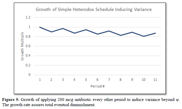
We demonstrate here by a very simple, hypothetical schedule with
naïve assumptions (so as to sketch out the principle). Rather than administer
our recommended dosage of 100mcg for every period, we shall administer twice
that (with the naïve assumption that it will give us twice the shrinkage in
growth as with 100 mcg), and administering this only every other period (and
thus the assumption that the growth for these intervening periods is the growth
rate, if left entirely untreated, of 1.08).
We sketch this hypothetical for illustrative purposes (Table 6).
And after 10 periods of
such alternating double-treatments, we find growth has been reduced by nearly
13%, depicted in Figure 9.
This simple, hypothetical schedule is but one schedule – an
infinite number are available and if
the host can sustain the schedule, then there exists a schedule of
administration more effective
than the accepted, outright, constant-blood level recommend dosages.
Mathematically, therefore, there exists many schedules that are more beneficial
provided the host can sustain the schedule.
We have been discussing the growth of bacteria in a petri dish,
but the same notion can be extended to a bacterial infection in a human being, e.g., an upper-respiratory infection
and antibiotic treatment. Again, the critical caveat is if the host can sustain the schedule being the limiting factor.
Different antibiotic treatments can be handled in varying doses differently,
and thus the principle of increasing the variance also affects which antibiotic
to invoke.
Further, not only is the principle applied with this
caveat to bacterial infections but other malevolent cell function conscriptions
as well, such as cancer and potential chemotherapy dosages and abilities to
sustain higher dosages, with some chemotherapies and doublets thereof more
easily sustained at the varying dosages than others, thus becoming of possibly
greater concern, ceteris paribus.
Example 3 – Pathogenic spread through a
population
Thus far we have looked at an example of an out of control
national debt, as well as certain infections and malevolent cellular
conscriptions within an organism. We can also apply these simple properties to
the growth function innate in a pathogenic outbreak between organisms
themselves. This too is a geometric growth function, and the effect of
increasing the period-on-period variance in growth to tame the function applies
as well.
Let us consider a population of organisms, human beings in the
immediate case, where a viral outbreak occurs. The problem in application of
these properties in all cases – not just the examples cited here in is
two-fold:
1. 1. How
can we induce greater period-on-period variance (i.e.,what actions can
we take to migrate rightward on the horizontal axis of Figures1,3,4,5,6,7, and
8)?
-and-
2.
Can we induce variance safely enough that we can achieve the
growth-terminal critical point ψ?
Inducing period-on-period variance can be achieved through various
possible measures with the one(s) best suited determined by qualified
epidemiologists. These, below, are a suggested sampling of possibilities:
1. Quarantine, much like an antibiotic or chemotherapy in
the malevolent cellular growth example, a sporadic period between serious, hard
lock-down and none-at-all.
2. Prophylactic measures (usually pharmacological) even if
only to segments of the population sporadically, to induce variance.
3. Vaccination - which, when applied to the entire
population, liberates the population from that pathogenic event, but even if to
only part of the population will induce variance.
These measures can provide a viable stop-gap for situations
involving limited resources if they induce enough variance in the
period-on-period growth rate of infected individuals within a population.
If we can induce variance in the spread of a pathogen within a
population and do so safely such that the invoked variance is of degree
sufficient to achieve the growth-terminal critical point ψ, the
growth curve is broken.
In the particular case of
attempting to invoke variance in period-on-period growth to mitigate the spread
of a pathogenic outbreak, it is vital to avoid entropic outcomes. That is to
say, if one measure is being used to induce variance, other measures must not
interfere in such. In inducing variance, a wave function is created on what
otherwise is a simple curved function of increasing spread. If multiple wave
functions are overlaid such that peaks and troughs cancel, which, conceivably
could occur if multiple avenues of inducing variance are invoked, especially in
uncoordinated fashion, the campaign to reduce the spread, to break the growth
function through increased period-on-period variance in growth, will fail.
CONCLUSION
We have demonstrated how increasing
variance in geometric growth rates can diminish geometric growth. We find here
the aspects in the underlying data that are related to the geometric growth
rate by a Pythagorean or closely-Pythagorean relationship, depending on the
distribution of outcomes. These three components are the arithmetic mean growth
rate, A, the geometric mean growth rate, and the variance (or standard
deviation in growth rates). When the arithmetic growth rate squared less the
resultant variance is 1 or less, the growth will ultimately cease (as
multiplying any product repeatedly by a number less than 1 yields a new product
approaching zero).
We
examined growth rates with respect to a fraction of resources to allocate to
risk, or in proxy of that, growth rates with respect to the cosine of the
standard deviation in period-on-period outcomes and their arithmetic average.
Often we only have the geometric average period-on-period growth rate, and must
sketch out what the variance or standard deviation is, as well as the
arithmetic average growth rate, and where this is not feasible, we must seek a
schedule of increasing variance until the growth-terminal
critical point ψ is arrived at.
We
have looked at examples which are either politically agnostic, or uses less
resources, or heterodox approaches than conventionally used for “bending the
curve” of malevolent geometric growth. We have examined simple, hypothetical
examples where this might be applied in terms of a nation’s aggregate debt, in
terms of malevolent cellular growth, and in terms pathological spread through a
population. Each example also is riddled with specific concerns, such as “can
the host survive increased, sporadic doses,” as well as avoiding entropic
outcomes in more social applications such as pathological spread in a
population.
The examples provided, though hypothetical and naïve to their field of application, are provided as trail heads, as a means of sketching out how one might go about attempting to find a means to apply the principle of increased variance and to highlight potential pitfalls to be avoided for the particular application.
Bernoulli, D.
(1738). Specimen theoriae novae de mensura sortis (Exposition of a new theory
on the measurement of risk). In Commentarii academiae scientiarum imperialis
Petropolitanae 5: 175-192. Translated into English: L. Sommer. Econometrica 22:
23-36.
Fisher, R.A.
(1930). The Genetical Theory of Natural Selection, Clarendon Press, Oxford.
de La Grandville.,
O. (1998). The Long-Term Expected Rate of Return: Setting It Right, Financial
Analysts Journal, November/December.
Latané, H.A.
(1959). Criteria for Choice among Risky Ventures. Journal of Political Economy 67(2).
Kelly, J. L.
(1956). A new interpretation of information rate. Bell System Technical Journal
35: 917-926.
Lopez de Prado,
M., Vince, R. & Zhu, Q. (2019). Optimal Risk Budgeting Under a Finite
Investment Horizon. Risks 7(3): 86.
Shannon., C.E.
(1948). A Mathematical Theory of Communication. Bell System Technical Journal
27: 379-423 & 623-656.
Thorp., E.O.
(1962). Beat the Dealer. Random House, New York,
Vince, R., (1990).
Portfolio Management Formulas. John Wiley and Sons, New York,
Vince, R. (1992).
The Mathematics of Money Management. John Wiley and Sons, Hoboken, NJ.
Vince, R. (1995).
The New Money Management: A Framework for Asset Allocation. John Wiley and
Sons, Hoboken, NJ.
Vince, R., (2012).
Risk-Opportunity Analysis. Kindle Publishing Division of Amazon,
Vince, R.
Expectation., & Optimal f., (2019). Far East Journal of Theoretical
Statistics 56(1), 69-91.
Vince, R &
Zhu, Q.J. (2013). Inflection point significance for the investment size. SSRN,
2230874.
Vince, R &
Zhu, Q.J. (2015). Optimal Betting Sizes for the Game of Blackjack. Journal of
Investment Strategies 4(4), 53-75.
-
 Table 1
 -
Table 2
-
Table 3
-
Table 4
-
Table 5
-
Table 6