Journal of Economics, Business and Market Research (ISSN: 2642-022X)

Research Article
THE MONETARY POLICY INSTRUMENTS AND INFLATION, ANALYSIS WITH A STRUCTURAL BREAK: AN APPLICATION TO ALGERIA
5489
Views & Citations4489
Likes & Shares
This study aims to study the development of inflation in the Algerian economy through monetary policy in addressing this phenomenon, and the data includes annual data covering the period from 1970 to 2019., based on macroeconomic variables which expose the relationship between the inflation and monetary policy instruments, the econometric study based on structural break cointegration, using a structural break tests such as Zivot and Andrews(1992) and Gregory-Hansen(1996) to estimate this relationship we used the cointegration methods “ FMOLS, DOLS, CCR” these estimation methods had allowed us to note that the treatment of inflation in Algeria is not based not only on monetary tools.
Keywords: Monetary Policy instruments, Inflation, Structural break cointegration, Algeria.
Jel classification Codes: E4. E5 .C24 .C34
Monetary policy is considered one of the most important tools to achieve general economic equilibrium, as it is one of the most widely used means in economic policy, but its success is linked to precision and good management of it. Monetary policy has taken an important place in the present times among other economic policies, and its role has become decisive in influencing various economic changes, and this is clearly demonstrated by the link with economic problems such as inflation and deterioration of local currencies with monetary solutions, the Money supply with the level of economic activity, and this includes monetary policy to influence inflation through the quantitative and qualitative tools of monetary policy (Woodford, M. 2001, Inflation is one of the indicators of the economic situation (Willard, L.2006), like any economic situation or phenomenon, and it is not necessarily considered a satisfactory condition as long as it does not exceed its limits, as well as inflation is necessarily a condition of health, because reading the reality of inflation to clarify what it refers to depends on the conditions that accompany it. is well known that inflation is an indicator behind which hides facts which can be positive or negative and, therefore, inflation must be brought under control before the level of risk becomes dependent on its causes, (Romer, & Romer, 1989). Inflation is an economic phenomenon that affects the economies of developing countries alike, and inflation increases in the economies of countries whenever there is an environment conducive to increasing inflationary pressures, the economy, which depends on its impact on a set of factors and variables that help fuel inflationary pressures and push domestic prices up. Inflation targeting requires the availability of an economic policy capable of combining and adapting different tools, and as part of this corrective process, we find that most of these countries seek in the first place to put economic policies in general and monetary policy in particular on the right track in order to be able to achieve the set objectives More precision, efficiency and more transparency.
LITERATURE REVIEW
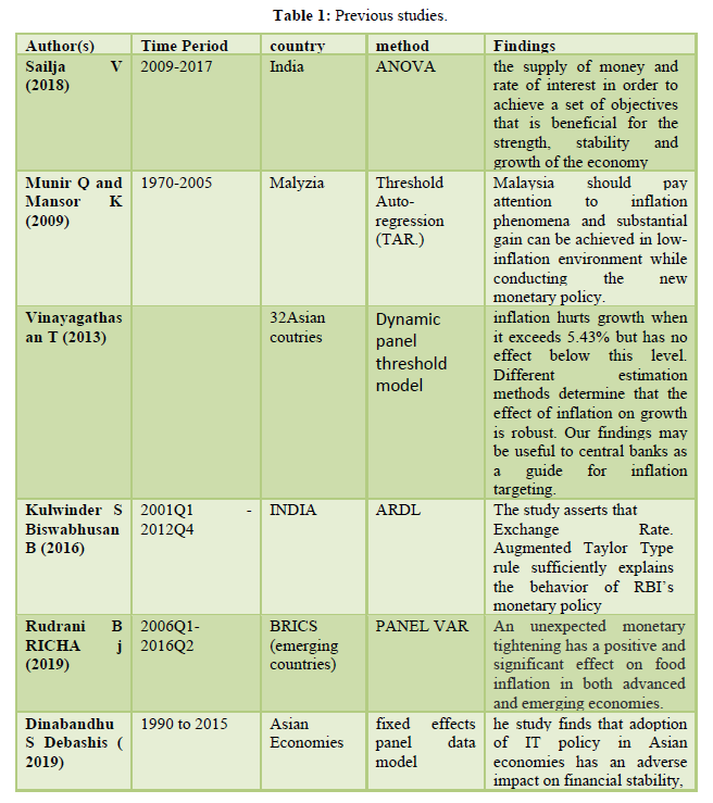
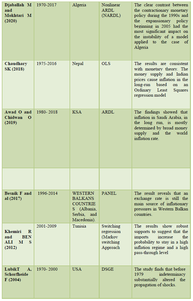
Recently, most studies have focused on break point cointegration approach and nonlinear relationships between variables, our review of the literature is limited to studies that focus on the joint inflation and monetary policy instruments which are highlighted in the table 1 below.
DATA AND MEDOTHOLOGY
This research adopts the public’s perspective in collecting the information which market participants receive from the central bank, among possible interest groups, financial market participants actively follow the news concerning central bank events and receive information which immediately drives market reactions, if the released communication is efficient. This study assumes that the financial crisis made central bank communication even more important as an information source for market participants, because economic conditions changed rapidly and new information was desperately needed to reduce the widening information gap between the central banks and market participants. (Blinder, Ehrmann, Fratzscher, De Haanand & Jansen, 2008) suggest that the response of financial markets to central bank communication is significantly larger under increased uncertainty than in “normal” times, speeches and interviews reported by international news agencies provide updated and frequent information and help in narrowing the information gap between monetary policy meetings, (Jensen, 2002) which are held yearly in the European central bank and eight times, (Gürkaynak, Refet, 2005) because of their high frequency and real-time content, news items concerning statements of policy-makers are widely followed in financial market, to analysis the impact of monetary policy on economic development in Algeria, the time serried data established by World Bank, world development indicator (WDI, 2019) and the annual time serried data from an annual economic report of the Bank Algeria from 1970-2019 have been taken to analyze the relationship between variables. The specific model can be formulated as below:
INF= 𝑓 (𝑀2, 𝑅E𝑅, IR,) (1)
To transform the above model (1) to a multiple regression form can be written like this:
INF= 𝛽0 + 𝛽1𝑀2 + 𝛽2𝑅E𝑅 + 𝛽3 + 𝜀 (2)
Where 𝑀2 is broad money, 𝑅E𝑅 is real exchange rate DZD /USD, 𝐼𝑅 is the interest rate, INF is inflation rate, 𝜀 is error term, 𝛽0 is intercept, 𝛽1, 𝛽2, 𝛽3, is the coefficient of the independent variable, in presence study we have used time series data, therefore, checking for stationary technique needs to apply to check whether all series stationary or not, regarding to the previous study found that most of the economic time series data are found to be non-stationary and a non-stationary time series may produce spurious regression, (Phillips & Perron,1988).
EMPIRICAL FINDINGS
The data set used for the empirical analysis in this paper consists of annual observations over the period of 1970-2019 in Algeria the inflation rate (INF) represents the dependent variable, (𝑀2) is broad money, 𝑅E𝑅 is real exchange rate DZD /USD, and finally (𝐼𝑅) is the interest rate,
Co integration analysis without accounting for structural Breaks
Prior to modeling time-series data, the order of the integration of the series has to be determined. The traditional unit root tests, namely, the Augmented Dickey-Fuller test (ADF) (Dickey & Fuller, 1981) and the Phillips-Perron test (PP) (Phillips & Perron, 1988) provide convenient procedures to determine the univariate properties of time-series data. The results of the unit root tests are presented in Table 2. It is evident that based on both ADF and PP tests; the null hypothesis of nonstationary cannot be rejected for all level data, an exception is PP without trend.
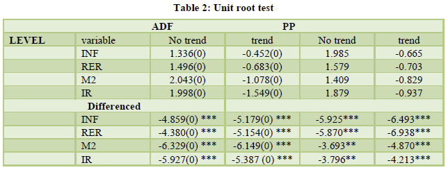
Notes: Numbers in parentheses are the numbers of the lags in the augmented term of the ADF regression. For both ADF and PP tests, (MacKinnon’s 1991) critical values are used to test the null of non-stationarity. ***, ** and *indicate the significance at 1%, 5% and 10% levels respectively.
Having established that all variables are integrated of the same order, we proceed with the Johansen multivariate cointegration tests (Johansen & Juselius, 1990) which allows us to test for long-run budget balance sustainability, to implement this procedure, an appropriate lag length in the Vector Autoregressive (VAR) model is determined as one by Akaike’s information criterion (AIC) and Schwarz Bayesian criterion (SBC).
Likelihood Ratio test of deletion of deterministic/exogenous variables in the VAR model shows that the model should include an intercept but not a trend. Table 3 reports the results of the Johansen’s cointegration tests. Maximum Eigenvalue and trace statistics reject the null hypothesis of no cointegration at 5 % significance level, the normalized value of the cointegrating vector (β) is 0,623, the over identifying restriction β=1 imposed on the cointegrating vector gives Chi-square (1) =196,81 with a p-value of 0,001, therefore, Johansen cointegration procedure suggests a cointegrating vector which does not statistically equal to one, with the conventional cointegration analyses, The result of weak sustainability might be due to the existence of a structural break. This leads us to pursue further testing using alternative procedures that can accommodate potential structural breaks in the data.
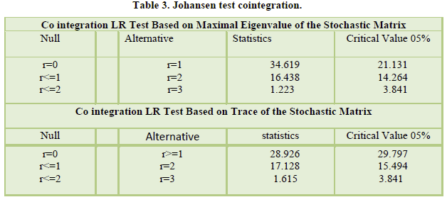
Notes: List of the variables included in the co integrated vectors and intercept; Order of VAR=1 and selected through Akaike’s information criterion (AIC) and Schwarz Bayesian criterion (SBC)
Cointegration Analysis with accounting for structural Breaks
Zivot and Andrews test
Problem common with the conventional unit root tests such as the ADF, DF-GLS and PP tests, is that they do not allow for the possibility of a structural break. Assuming the time of the break as an exogenous phenomenon, Perron showed that the power to reject a unit root decreases when the stationary alternative is true and a structural break is ignored. Zivot and Andrews propose a variation of Perron’s original test in which they assume that the exact time of the break-point is unknown. Instead, a data dependent algorithm is used to proxy Perron’s subjective procedure to determine the break points. Following Perron’s characterization of the form of structural break, Zivot and Andrews proceed with three models to test for a unit root: (1) model A, which permits a one-time change in the level of the series; model B, which allows for a one-time change in the slope of the trend function, and model C, which combines one-time changes in the level and the slope of the trend function of the series. (Narayan and Stephan 2010) Hence, to test for a unit root against the alternative of a one-time structural break, Zivot and Andrews use the following regression equations corresponding to the above three models.

where DUt is an indicator dummy variable for a mean shift occurring at each possible break-date (TB) while DTt is corresponding trend shift variable. Formally
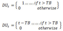
The null hypothesis in all the three models is α=0, which implies that the series {yt} contains a unit root with a drift that excludes any structural break, while the alternative hypothesis α
The results for Zivot and Andrew unit root test are presented in Table 4 Since the dummy variables in Model C are not significant for our empirical models, we exclude the Model C meaning that there’s no simultaneous mean and slope shift in our variables. Since the dummy variables in Model C are not significant for our empirical models, we exclude the Model C meaning that there’s no simultaneous mean and slope shift in our variables. These results suggest that we can reject the null of unit root for our variables at 5 percent significance.
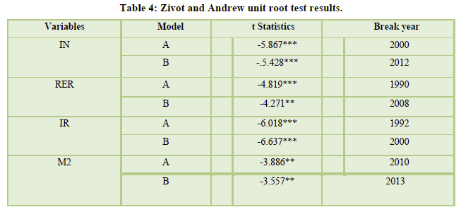
The critical values for Zivot and Andrews test are -5.57, -5.30, -5.08 and -4.82 at 1 %, 2.5 %, 5 % and 10% levels of significance respectively. * denotes statistical significance at 5% level. ** denotes statistical significance at 10% level.
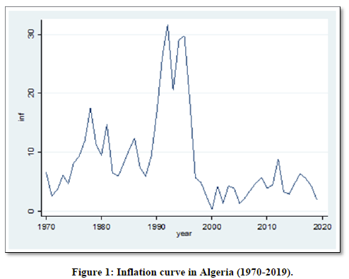
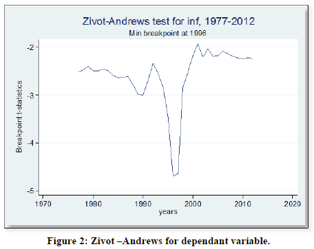
Generally, the years 1992 ,1996 .2012 are switching years when the country disunited into two sovereign states, is regarded as the most suitable candidate for a structural break in Algeria, the results show that only one of the four series studied (i.e.) near witness to the presence of a structural break in1990(the laws of money and credit). Contrary to prevailing perception, the test identifies a break in the inflation series at 2000, the results also show that the year 2013 stands out as the flag of the return of the increase in the price of oil and its reflection on the monetary policy in Algeria (Figure 2).
Gregory-Hansen co integration test:
The test for co integration in the presence of an unknown structural break, we used the cointegration tests suggested by Gregory and Hansen (1996), a structural change would be reflected in a change in the intercept and/or a change in the slope. Gregory and Hansen (1996) use four different models as below:
Model 1: Level Shift (C)
 (6)
(6)This is a simple case in which there is a level shift in the cointegrating relationship, modeled as a change in the intercept , where the slope coefficients are held constant. This implies that the cointegration relationship has shifted in a parallel fashion, in this parameterization , represents the intercept before the shift and represents the intercept after the shift.
Model 2: Level Shift with Trend (C/T)
 (7)
(7)Where is the coefficient of the trend term, t.
Model 3: Regime Shift (C/S)
 (8)
(8) Denote the co integrating slope coefficients before the regime shift and denote the change in the slope coefficients. In principle, the same approach used in equations could be used for testing models (1) to (4) if the timing of the regime shift were known a priori. However, such breakpoints are unlikely to be known in practice without some appeal to the data. Within this framework, Gregory and Hansen (1996) proposed the test for cointegration with an unknown break date, which involves computing the usual statistics (ADF and Philips test statistics) for all.
Possible break points and then selecting the smallest values, since this will potentially present greater evidence against the null hypothesis of no cointegration. In this regard, the relevant statistics are the ADF ( ), and
Model 4: Regime shift with trend (C/S/T)
 (9)
(9)In this case the structural break affects Lee, J., and Strazicich M (2001), all the components of series intercept, slope and trend.
The results for Gregory- Hansen test are presented in Table 5.
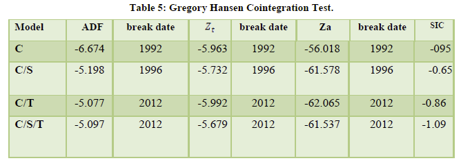
The 5 percent critical values for ADF (and Z t) are -5.56, -5.83 and -6.41 for models respectively while the Za for the same equations are –59.40, -65.44 and-78.52, respectively (Table 1 of Gregory and Hansen, 1996) ** indicates the existence of co integration at 5% level.
This result confirms that long run relationship exists among inflation, monetary policy tools money supply, exchange rate spread and interest rate, it shows that co integration is established under the assumption of shifts in both the level and the slope with the shift occurring in 1992, 1996, and 2012 with minimum SIC. Having established a structural break in 2000, the indicator function = 0 for periods 1970: to 2012 and=1 for periods after 2012, the results of the estimated implied Gregory and Hansen equation.
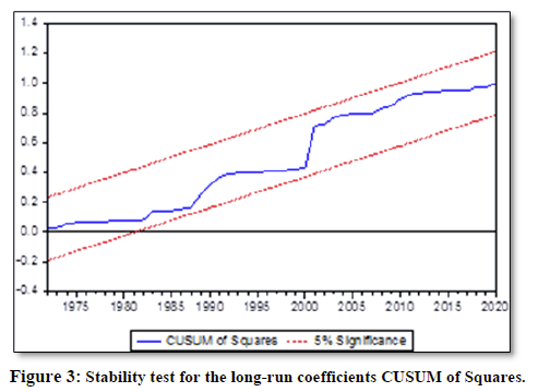
To determine the long-run coefficient among the variables under review is crucial. This study adopted the FMOLS, DOLS and CCR as tools to investigate the magnitude of the cointegration relationship among the four variables, all co integration regression tests (FMOLS, DOLS, and CCR) are in harmony in terms of statistical significance and sign orientation and the CUSUM tests show the stability of the estimated model, we observe from Table 6 that.
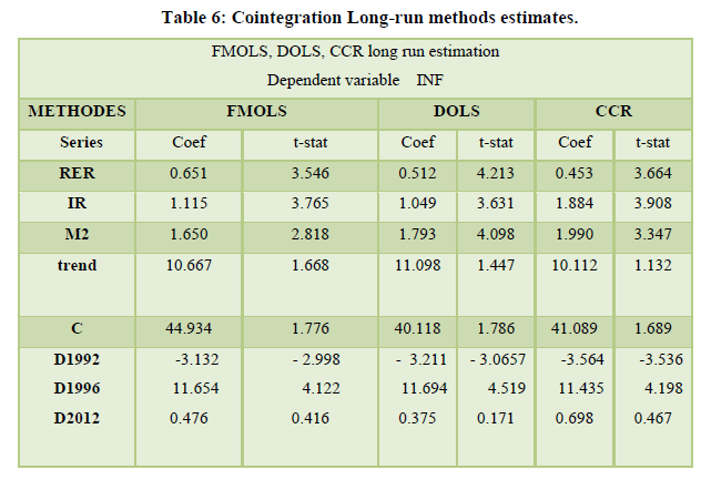
For the final step of our empirical analysis, the methodology of Stock and Watson (1993) is used to estimate the cointegrating vector involving deterministic components. The estimators can be computed using OLS and called as dynamic OLS estimators (DOLS), fully modified OLS (FMOLS) estimators and canonical cointegrating regression estimators (CCR) perform better comparatively to other asymptotically efficient estimators especially in small samples, the estimation results are presented in Table 6. The t-statistics of estimators indicate that the dummy variables are statistically different from zero. In addition, testing the restriction of the null hypothesis β=1, we get: chi-square (1) = 723.273 [p-value=0.00], which implies that the inflation in Algeria explained by monetary policy instruments (Figure 3).
CONCLUSION
Our empirical results emphasize a significant direct relation inflation between and the monetary instruments such as interest rate, real exchange rate and
M2, which make interest rate an efficient instrument for central bank to prevent inflation, we can a state that protecting interest rate is a lever for inflation targeting strategies; also, there is is an inverse statistically significant relation between the inflation rate, the results revealed the presence of a significant long-run relationship between the variables the structural breaks all long-run regression results of FMOLS, DOLS and CCR confirmed that the monetary policy tools exert a inelastic statistically significant relationship on inflation over the sampled period, this indicates that the inflation rate is one of the objectives of monetary policy is committed to expand on the main structural variables and causal relations involved in guaranteeing a state of equilibrium, by offering to the monetary theory and practice the possibility of choosing and logically connecting macroeconomic variables, for many analysts, monetary policy still owes a solution to recession. In a global framework of financial interdependence and increased uncertainty, the monetary policy should ideally be characterized by commitment, consistency, dynamics, transparency, accountability, quality assessment and avoidance of excessive fluctuation and flexibility; set of attributes that inevitably involve a high degree of complexity.
- Awad, O., & Shidwan, O. (2019). Investigating the Causes of inflation in Saudi Arabia: An Application of Autoregressive Distributed Lag (ARDL) Model. International Journal of Applied Engineering Research 14(21): 3980-3986.
- Besnik, F, Paul, S.K., Agron, C, & Ariana, F. (2017). The relationship between exchange rate and inflation: The case of western balkans countries. Journal of Business, Economics and Finance 5(4).
- Blinder, A.S, Ehrmann, M, Fratzscher, De, Haanand, D.J. & Jansen, J. (2008). Central bank comunication and monetary policy a survey of theory and evidence, working paper series 898.
- Chaudhary, S.K. (2018) Analysis of the Determinants of Inflation in Nepal. American Journal of Economics 8(5): 209-212.
- Dickey, D.A., & Fuller, W.A. (1981). Likelihood Ratio Statistics for Autoregressive Time Series with a Unit Root, Econometrica 49(4),1057-1072.
- Dinabandhu, S. & Debashis. (2019). Monetary Policy and Financial Stability: The Role of Inflation Targeting. Australian Economic Review 53(1), 50-75.
- Djaballah. M, & Mokhtari, M. (2020). Analysis of asymmetry between velocity of money and inflation in Algeria. Journal of Business Administration and Economic Studies 6(1), 201-216.
- Gregory, A. & Hansen, B. (1996). Residual Based Tests for Cointegration in Models with Regime hifts, Econometrica 70, 99-126.
- Gürkaynak, & Refet, S. (2005). Using Federal Funds Futures Contracts for Monetary Policy Analysis (FEDS Working peper.
- Gürkaynak, & Refet, S. (2005). Using Federal Funds Futures Contracts for Monetary Policy Analysis. Federal Reserve Board, Finance and Economic Discussion Series 29.
- Jensen, H. (2002.). Optimal Degrees of Transparency in Monetary Policy Making. Scandinavian Journal of Economics, 104(3), 399-422.
- Jensen, H. & Beetsma, R. (2002). Monetary and fiscal policy interactions in a micro-founded model of a monetary union Working Paper Series 166, European Central Bank. Handle: RePEc: ecb: ecbwps: 200216.
- Johansen, S., & Juselius, K. (1990). maximum likelihood estimation and inference on cointegration with applications to the demand for money First published. https://doi.org/10.1111/j.1468-0084.1990.mp52002003.x
- Kapetanios, G. (2005). Unit-root testing against the alternative hypothesis of up to m structural breaks. Journal of Time 26(1), 123-133.
- Khemiri, R., & Benali, M.S. (2012). Exchange Rate Pass-Through and Inflation Dynamics in Tunisia: A Markov-Switching Approach. Economics Discussion Papers 20, 12-39.
- Kulwinder, S., & Biswabhusan., B. (2016). Estimating Taylor Type Rule for India's Monetary Policy using ARDL Approach to Co-integration. Indian Journal of Economics and Development 12(3): 515-520.
- Lee, J., & Strazicich., M. (2001). Break Point Estimation and Spurious Rejections with Endogenous Unit Root tests. Oxford Bulletin of Economics and Statistics 63(5), 535-558.
- Lubik, T, A., & Schorfheide., F. (2004) Testing for Indeterminacy: An Application to U.S. Monetary Policy. American Economic Review 94(1), 190-217.
- Munir, Q., & Mansour., K. (2009). Non-Linearity between Inflation Rate and GDP Growth in Malaysia. Economics Bulletin 29(3), 1555-1569.
- Narayan, P.K. & Stephan, P. (2010). A New Unit Root Test with Two Structural Breaks in Level and Slope at Unknown Time. Journal of Applied statistics 37(7).
- Phillips, P.C.B., & Perron, P. (1988). Testing for a Unit Root in Time Series Regression. Biometrika 75(2), 335-346.
- Romer, C., & Romer, D. (1989). Does Monetary Policy Matter? A New Test in the Spirit of Friedman and Schwartz. In NBER Macroeconomics Annual 1989, Olivier Jean Blanchard and Stanley Fischer. Cambridge (MA): MIT Press 121-170.
- Rudrani, B., & Richa, J. (2019). Can monetary policy stabilise food inflation? Evidence from advanced and emerging economies. Economic Modelling 89, 122-141.
- Sailaja, V. (2018). A Study on Impact of Monetary Policy on GDP and Inflation. Journal of Advance Research in Dynamical &Control Systems 10(8), 197-203.
- Sen, A, (2003). On Unit-Root Tests When the Alternative Is a Trend-Break Stationary Process. Journal of Business & Economic Statistics, American Statistical Association 21(1), 174-184.
- Stock, J.H., & Watson, M.W. (1993). A Simple Estimator of Cointegrating Vectors in Higher Order Integrated Systems. Econometrica 61(4), 783-820.
- Vinayagathasan, T. (2013). Inflation and economic growth: A dynamic panel threshold analysis for Asian economies Journal of Asian. Economics 26, 31-41.
- Vogelsang, T., & Perron, P. (1998). Additional Tests for a Unit Root Allowing for a Break in the Trend Function at an Unknown Time. International Economic Review 39(4), 1073-1100.
- Willard, L. (2006). The Effect of Inflation Targeting on Inflation: A Reassessment, Ph.D. dissertation essay, Princeton University.
- Woodford, M. (2001). Monetary Policy in the Information Economy. In Economic Policy for the Information Economy. Kansas City: Federal Reserve Bank of Kansas City 297-370.
- World Bank WDI (2019) Available online at: https://data.worldbank.org/country/algeria?view=chart
- Zivot, E. & Andrews, D.W.K. (1992). Further Evidence on the Great Crash, the Oil-Price Shock, and the Unit-Root Hypothesis. Journal of Business & Economic Statistics 10(3), 251-270.
-
 Table 1
 -
Table 2
-
Table 3
-
Table 4
-
Table 5
-
Table 6
-
Table 7


